Activation functions in neutral networks

The Back propagation algorithm allows multilayer feedforward neural networks to learn input/output mappings from training observations. Backpropagation in neural networks adapts themselves to learn the relationship between the set of example patterns that could be leveraged to apply the same relationship to new input patterns. The network is able to focus on the features of an arbitrary input. The activation function is used to transform the activation level of a unit (neuron) into an output signal. There are a number of common activation functions in use with artificial neural networks (ANN). This paper aims to perform an analysis of the different activation functions and provide a benchmark of it. The purpose is to figure out the optimal activation function for the problem of predicting flight delays or no delays for Hawaiin Air flights. This further intends to help in better planning and control of disruption management.  

Introduction:

Neural networks are a set of algorithms, modeled loosely after the human brain, that is designed to recognize patterns. They interpret sensory data through a kind of machine perception, labeling, or clustering raw input. The patterns they recognize are numerical, contained in vectors, into which all real-world data, be it images, sound, text, or time series, must be translated. A neural network is called a mapping network if it is able to compute some functional relationship between its input and output. For example, if the input to a network is the value of an angle, and the output is the cosine of the angle, the network performs the mapping θ→ cos(θ). Suppose we have a set of P vector pairs (x1,y1),(x2,y2),….,(xn,yn) which are examples of a functional mapping y = φx: x  R N, y  RM.  We have to train the network so that it will learn an approximation o = y' = φ' x.

It should be noted that learning in a neural network means finding an approximate set of weights. Function approximation from a set of input-output pairs has numerous scientific and engineering applications. Multilayer feed-forward neural networks have been proposed as a tool for nonlinear function approximation [1], [2], [3]. Parametric models represented by such networks are highly nonlinear. The backpropagation (BP) algorithm is a widely used learning algorithm for training multilayer networks by means of error propagation via variational calculus [4], [5]. It iteratively adjusts the network parameters to minimize the sum of squared approximation errors using a gradient descent technique. Due to the highly nonlinear modeling power of such networks, the learned function may interpolate all the training points. When noisy training data are present, the earned function can oscillate abruptly between data points. This is clearly undesirable for function approximation from noisy data.

Fundamental of Propagation

Backpropagation is an algorithm used to train neural networks, used along with an optimization routine such as gradient descent. Gradient descent requires access to the gradient of the loss function with respect to all the weights in the network to perform a weight update, in order to minimize the loss function. Backpropagation computes these gradients in a systematic way. Backpropagation along with Gradient descent is arguably the single most important algorithm for training Deep Neural Networks and could be said to be the driving force behind the recent emergence of Deep Learning. Any layer of a neural network can be considered as an Affine Transformation followed by the application of a non-linear function. A vector is received as input and is multiplied with a matrix to produce an output, to which a bias vector may be added before passing the result through an activation function such as sigmoid.                 

Input=x                 
Output=f(Wx+b)

Consider a neural network with a single hidden layer like this one. It has no bias units. We derive forward and backward pass equations in their matrix form.

The forward propagation equations are as follows:

Input=x0
Hidden Layer1 output=x1=f1(W1x0)
Hidden Layer2 output=x2=f2(W2x1)
Output=x3=f3(W3x2)
To train this neural network, we could either use Batch gradient descent or stochastic gradient descent. Stochastic gradient descent uses a single instance of data to perform weight updates, whereas the Batch gradient descent uses a complete batch of data.

For simplicity, let's assume this is a multi-regression problem. Stochastic update loss function:

    Batch update loss function:

Here t is the ground truth for that instance.

We will only consider the stochastic update loss function. All the results hold for the batch version as well.

Let us look at the loss function from a different perspective. Given an input x0, output x3 is determined by W1, W2, and W3. So the only tuneable parameters in E are W1, W2, and W3. To reduce the value of the error function, we have to change these weights in the negative direction of the gradient of the loss function with respect to these weights.

                w=w−αw*∂E/∂w    for all the weights w

Here αw is a scalar for this particular weight, called the learning rate. Its value is decided by the optimization technique used. Backpropagation equations can be derived by repeatedly applying the chain rule. First, we derive these for the weights in W3:

Here ∘ is the Hadamard product.
Let's sanity checks this by looking at the dimensionalities. ∂E/∂W3 must have the same dimensions as W3. W3’s dimensions are 2×3. Dimensions of (x3−t) are 2×1 and f′3(W3x2) is also 2×1, so δ3 is also 2×1. x2 is 3×1, so dimensions of δ3xT2 are 2×3, which is the same as W3.     
Now for the weights in W2:

Let's sanity check this too. W2’s dimensions are 3×5. δ3 is 2×1 and W3 is 2×3, so WT3δ3 is 3×1.           f′2(W2x1) is 3×1, so δ2 is also 3×1. x1 is 5×1, so δ2xT1 is 3×5. So this checks out to be the same.   
 
Similarly for W1:

We can observe a recursive pattern emerging in the backpropagation equations. The Forward and     Backward passes can be summarized as below:
The neural network has L layers. X0 is the input vector, xL is the output vector and t is the truth vector. The weight matrices are W1,W2,..,WL and activation functions are f1,f2,..,fL.

Forward Pass:

    Backward Pass:

Weight Update:

Equations for Backpropagation, represented using matrices have two advantages.
One could easily convert these equations to code using either Numpy in Python or Matlab. It is much closer to the way neural networks are implemented in libraries. Using matrix operations speeds up the implementation as one could use high-performance matrix primitives from BLAS. GPUs are also suitable for matrix computations as they are suitable for parallelization. The matrix version of Backpropagation is intuitive to derive and easy to remember as it avoids the confusing and cluttering derivations involving summations and multiple subscripts.

Types of activation functions

     3.1    Identity     
Also known as a linear activation function.

3.2    Step

3.3  Piecewise Linear

Choose some xmin and xmax, which is our "range". Everything less than this range will be 0, and everything greater than this range will be 1. Anything else is linearly-interpolated between. Formally:

Where
m=1/xmax−xmin
and
b=−mxmin=1−mxmax

3.4   Sigmoid

3.5  Complementary log-log

3.6   Bipolar

3.7  Bipolar Sigmoid

3.8  Tanh

3.9  LeCun's Tanh

Scaled:

3.10   Hard Tanh

3.11   Absolute

3.12   Rectifier

Also known as Rectified Linear Unit (ReLU), Max, or the Ramp Function.

Modifications of ReLU

These are some activation functions that have been discovered over time :

Scaled

Scaled:

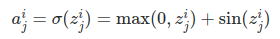
3.13  Smooth Rectifier

Also known as Smooth Rectified Linear Unit, Smooth Max, or Soft plus

3.14   Logit

3.15   Probit

Where erf is the Error Function. It can't be  described via
elementary functions,

Alternatively, it can be expressed as

Where ϕ is the Cumulative distribution function (CDF).

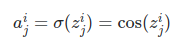
3.16   Cosine




3.17     Softmax

Also known as the Normalized Exponential.

3.18    Maxout

Essentially the idea is that we break up each neuron in our maxout layer into lots of sub-neurons, each of which has their own weights and biases. Then the input to a neuron goes to each of its sub-neurons instead, and each sub-neuron simply outputs their z's (without applying any activation function). The aim of that neuron is then the max of all its sub-neuron's outputs.

Formally, in a single neuron, say we have n sub-neurons. Then

where

Experiment setup &  results:

A dataset was chosen for the evaluation of the activation network. A simulator was specially developed for testing the activation function using an open-source library FANN (Fast Artificial Neural Network). The simulator was developed in Python and language bindings for FANN were used which itself was created using SWIG (Simplified Wrapper Interface Generator). T The business case that this paper tries to solve is of Disruption Management for Hawaiin Airlines. The dataset has been created after merging two different types of raw data related to flights and weather obtained from the following sources for flights operating from Honolulu airport for Hawaiin Airlines -

a) Flights Statistics & operations data obtained from the Bureau of Transportation Statistics (https://www.bts.dot.gov/)
b) Weather information obtained from Wunderground (https://www.wunderground.com/)

The problem presented here is of binary classification that predicts whether a Hawaiin Airflight operating from Honolulu would be delayed or not based on the dataset fed into FANN. 36 different features like Flight Time, Aircraft Type, Time of flight, Ground Operations, Temperature, Humidity, Air pressure among others were fed into the input layer of FANN.  These 36 features were converted into 122 different neurons on the basis of implicit feature engineering carried out by 4 separate hidden layers.

At the output layer, the sigmoid function is used to derive the probabilities of prediction for binary classification.

Conclusion:

The activation function is one of the essential parameters in a Neural Network. The performance evaluation of different activation functions shows up that the selection of an activation function plays an important role in faster convergence and minimalization of the error, thereby, enhancing the network performance and increasing prediction accuracy. As shown in the table above, Leaky Relu and Relu outperforms other activation functions by a good error margin (though Leaky Relu performs better than Relu only marginally).

This paper emphasizes that although the selection of an activation function for a neural network or it's node is an important task, other factors like training algorithm, network sizing, and learning parameters are also vital for proper training of the network.

References:

 [1] K. Homik, M. Stinchcombe, and H. White, “Multilayer feedforward networks are universal approximators”, Neural Networks, vol. 2, pp.359-366, 1989.
    [2] C. Ji, R. R. Snapp, and D. Psaltis, “Generalizing smoothness constraints from discrete samples”,  Neural  Computation, vol. 2, pp. 188-197, 1990.
    [3] T. Poggio, and F. Girosi, “Networks for approximation and learning.” Proc. IEEE. vol. 78, no. 9, pp. 1481-1497. 1990.
    [4] Y. Le Cun, “A theoretical framework for backpropagation”, in Proc.1988 Connectionist Models Summer School, D. Touretzky, G. Hinton, and T. Sejnowski, Eds. June 17-26, 1988. San Mateo, CA: Morgan Kaufmann, pp. 21-28.
    [5] D. E. Rummelhart, G. E. Hinton. and R. J . Williams. “Parallel Distributed Processing: Explorations in the Microstructure of Cognition”, vol. I. MIT Press, ch. 8.
    [6] James A. Freeman and David M. Skapura. “Neural Networks Algorithms, Applications, and Programming Techniques”, pp 115-116, 1991.
    [7] Jacek M. Zurada, "Introduction to Artificial Neural Systems", pp 32-36, 2006.
    [8] Sudeep Raja, “A Derivation of Backpropagation in Matrix Form”, blog.